Units of measurement, symbols, significant digits and rounding off
1.1 Units of measurement and symbols
1.2 Significant digits
1.3 Rounding off
1.4 Bias, accuracy and precision
Individual Trees and Logs
2.1 Bole characteristics
2.1.1 Diameter
2.1.2 Height
2.1.3 Bark thickness
2.1.4 Volume
2.1.5 Stem form and taper
2.2 Log characteristics
2.2.1 Diameter
2.2.2 Length
2.2.3 Volume
2.2.4 Weight
2.2.5 Allowance for defect
2.3 Crown characteristics
2.3.1 Width
2.3.2 Depth
2.3.3 Surface area
2.3.4 Volume
2.3.5 Biomass
2.4 Stem analysis
Groups of Trees (Stands)
3.1 Number of trees
3.2 Diameter
3.3 Basal area
3.3.1 Fixed-area plots
3.3.2 Angle count sampling
3.3.3 Advantages and disadvantages of angle count sampling
3.4 Height
3.4.1 Mean height
3.4.2 Predominant height, top height, dominant height
3.4.3 Stand height curve
3.5 Volume
3.6 Crown closure
3.7 Crown biomass
3.8 Growth and increment
References
Appendix 1: Checklist of equipment and materials
[RWG#2] [Copyright] [Title Page] [Next Page] [Last Page]
3.3.2 DERIVING G - USING ANGLE COUNT SAMPLING
The principle of PPS sampling has been applied to various forest sampling problems but most notably to estimating G by angle counting where inclusion of a tree in the count depends on the basal area of the tree and its proximity to the sample point. The procedure is simple, quick and cheap to apply, but applying it properly requires considerable skill and a thorough understanding of the many sources of error likely to affect the estimate.
Collectively, the instruments used in ACS are termed angle gauges, the best known and most widely applied of which are the Spiegel Relaskop and wedge prism. Because of its exceptional versatility and other features, the Relaskop is particularly appropriate for forest inventory, whereas the low cost of the wedge prism makes it ideal for controlling silvicultural operations, e.g. monitoring the basal area that is both removed in thinning and left after it.
Apart from cost, the wedge prism has two advantages over the Relaskop. Firstly, only two lines need to be aligned to decide whether a tree is 'in' or 'out' and, secondly, slight movement of the tree or instrument does not interfere with the alignment - the tree and its image remain in the same relative position. Thus, the wedge prism is sometimes claimed to be faster and more accurate than the Spiegel Relaskop. In dense stands however, a problem may be experienced with the prism in matching the images to the trees from which they derive! This problem is easily overcome by rotating the prism through 90°ree; in the vertical plane which causes each image to 'return' to 'its' tree .
Controlling the many sources of error likely to affect estimates derived from ACS requires careful attention to the procedures described in Section 3.3.2.1.
3.3.2.1. Controlling Error in Angle Count Sampling
The procedures for controlling error in angle count sampling are grouped below into three categories related to (a) general matters, (b) the wedge prism, and (c) the Spiegel Relaskop .
(a) General
- Train the user to recognise when a tree is 'borderline' (applies to any angle gauge). This is best done by measuring the diameters of a number of trees, calculating the limiting distance for each using the appropriate formula (wedge prism - Formulas 19 or 20; standard metric Relaskop - Formula 22), and then viewing each tree from the appropriate limiting distance.
- Use a team of two persons comprising an assessor and an assistant. Have the assistant carry a 'T' piece around the periphery of the area being swept to define the DBH point on any doubtful tree, to help check any tree still doubtful after using the T-piece (see later), and to ensure that trees are not missed in the sweep. The assistant should also tally the count: this may include recording the species, crown classification, and bole quality, etc. of each counted tree.
- Select a distinctive tree or other fixed object, e.g. boulder, to define the start and finish of each sweep.
- If a tree is obviously unrepresentative at breast height, select a representative point and sight to it. Record this diameter as the dbh and record the height above ground at which it was taken.
- On all trees whether vertical or leaning, sight to breast height in a plane at right angles to the long (central) axis of the bole. Judge the breast-high level by eye unless the tree is doubtful (see next below).
- Check all doubtful trees by direct measurement and derive the limiting distance determining whether a tree is 'in' or 'out' (the formulas are presented later). Remember that ACS is frequently used in resource inventory where the intensity of sampling is often much less than 0.1%, i.e. one tree in a sweep actually represents at least 1000 trees in the population. If that one tree is a 'doubtful' tree and if it is worth, say, $30 on the stump, then $30 000 hinges on the decision whether the tree is 'in' or 'out'. Obviously, such a decision should be made with care!
- On average, the number of 'doubtful' trees in a sweep should not exceed 10% of the total count. A higher percentage than this suggests that the operator either has eyesight or other health problems, is inexperienced, or is unwilling to make a decision. Further training or a medical check may be required. Assessors inexperienced in using a Relaskop might try mounting the instrument on a tripod or other support for a day or two. Prolonged use of a tripod is undesirable as it is time consuming.
- To avoid missing trees when sweeping in dense stands of plantation grown trees, proceed with the sweep row by row.
- Trees wrongly counted in a sweep lead to an error in estimating G equal to the basal area factor (BAF) in m2/ha. Thus, one must compromise when selecting the BAF to use. Using a small factor gauge in a dense stand results in a large count and a greater likelihood of making a wrong count (missing a tree, etc.) but a relatively small error if a miscount is made. Conversely, a large factor gauge results in a small count and less likelihood of making a wrong count but a large error if a miscount is made. A satisfactory compromise is a count of 7-12 trees per sample point. Considering that in Australian forests, the basal area per hectare of fully stocked stands frequently lies between 20-50 m2/ha, BAFs of 2 to 5 should be appropriate in most situations. However, in heavily thinned stands and young poorly stocked forests, basal areas of 10-20 m2/ha are common. Thus, BAFs of 1 to 2 would be more appropriate.
- If a full 360°ree; sweep is not possible at a sample point near the forest boundary, determine G at the point by applying the practical and unbiased methods of either Grosenbaugh (1958) or Schmid-Haas (1982) . Grosenbaugh's method involves using a 180°ree; sweep if near a side boundary and a 90°ree; sweep if in a corner, and then weighting the estimate accordingly (x2 or x4).
- Be wary of the bias which can arise with eccentric and leaning stems. The former is the more serious but nothing can be done about it. One hopes that in a full sweep the errors will compensate. With a leaning stem, align the 'measuring' edge of the gauge at right angles to the longitudinal axis of the stem. Be particularly careful with trees which lean towards or away from the observer, especially if they are near 'borderline'. In this case, measure the slope distance from the sample point to the centre of the tree at ground level.
- When one tree is obscured by another, move sideways on the radius keeping the horizontal distance from the subject tree constant until the tree is clearly in view. Then make the reading and return to the sample point.
- Be alert for dead trees which normally are excluded from assessment.
- In mixed species forests, record the species of each tree counted to enable separate estimates of G to be made for each species as well as overall.
- If an estimate of the average basal area (G - ) of a forest stand (or compartment, etc.) is required, locate within the stand a number of sample points chosen either at random or systematically (e.g. superimpose a grid of an appropriate scale on a map of the area and sample at the grid intersections). If the structure of the forest is heterogeneous, stratify the forest prior to assessment and select an angle gauge of appropriate strength for each stratum (see next below). Use the same strength gauge throughout a stratum: doing otherwise causes problems later when analysing the data.
- To select an appropriate gauge for a forest tract, undertake a quick reconnaissance survey of G - within the tract using 5-7 subjectively chosen but well dispersed sampling points. Select any gauge, preferably one with a BAF between 2 and 4 m2/ha, and undertake a sweep at each point. From the 5-7 estimates of G derive G - and then apply the formula:

where F (m2/ha) is the BAF required. Select for the main survey an angle gauge whose BAF most closely approximates F . Adopting this procedure should give an average count of approximately 10 trees per sample point.
- Beware of operator bias when locating sample points in the field. Pacing the distance between successive points may be permissible provided one does not veer away from the specified bearing or alter one's pace to prevent the sample point falling, say, on a rocky knoll, in a creek bed, or within a large clump of nettle. To avoid such bias, pace out the major part of the distance but measure the last 30 metres or so by tape, keeping to the desired bearing throughout .
- Statistically speaking, each point within a forest qualifies as an independent sample point for ACS, i.e. two points only a metre apart could provide two independent estimates of basal area for a given stand even though the trees included in both samples may be identical or differ by only one or two trees. In practice, however, it is prudent to prevent such overlap. This is done by specifying in advance of the survey that the distance between plot centres must be more than double the limiting distance of the largest trees likely to be encountered in the stand (refer Formulas 19, 20 or 22).
- If information on the variability of G within a tract of forest is unknown, a rough guide to the number of sample points required in ACS to give a precise estimate of G - in reasonably uniform forest (most plantation stands) is:
Area (ha) No. of Sample Points
For more variable stands or if a highly precise estimate of G - is required, the number of sample points should be increased.
0.5 - 2.0 8
2.0 - 10.0 12
over 10.0 16
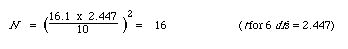
- For most efficient sampling, a quick reconnaissance survey of the forest is necessary as described above to give a rough estimate of the coefficient of variation (CV) of G. The actual number of sample points required can then be derived from the formula:

where N = estimated number of samples
C = coefficient of variation (%) of G derived from the reconnaissance survey
t = Student's-t value appropriate for the number of dfs attached to the pilot sample and the desired confidence level
E = the specified error limits (desired s.e. of the estimate) (%).
Thus, a quick pilot survey based on 7 sample points well distributed over an area to be assessed may indicate a G - of 32.4 m2/ha with a standard deviation of 5.21 m2/ha. Thus, C = 100 (5.2132.4 ) = 16.1%. Assuming that the error limit (E) is specified as ±10% at the 95% level of confidence, the number of sample points (N) required in the main survey is:
- To avoid error when sighting through the prism, hold it vertical at any convenient distance from the eye and perpendicular to the line of sight to the tree, and view the tree through its centre. Fixing the prism in a sighting tube of approximate diameter 45 mm and length 300 mm eliminates these likely sources of error. It also protects the prism from scratching, minimises smudging of the lens surface, confines the field-of-view to the tree under observation, and makes the prism easier to handle (and find).
- When making a judgement using a prism, keep it (not the observer's eye) vertically above the sample point or angle count spot as it is often called (note that the reference angle is generated at the surface of the prism whereas, with the Relaskop, it is generated at the eye) .
- Check any 'doubtful' tree by measuring d, the diameter of the tree overbark at breast height, and D, the measured slope distance from the sample point to the centre of the tree, and calculating for the BAF of the prism the maximum or limiting distance (LD) from the sample point within which a tree of that d is counted. Then compare this calculated limiting distance with the measured distance (D).

Prepared 'borderline tables' or a scientific calculator are essential for conducting this check efficiently.
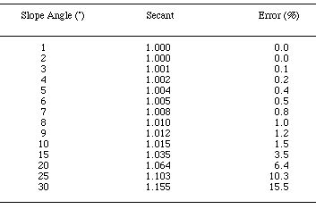
- On completing a sweep on sloping ground, correct the basal area estimate to horizontal by multiplying it by the secant of the maximum angle of slope (Ø) recorded through the sample point spot , viz.:

Correction for slope can be done in other ways (Barrett and Nevers, 1967) but all have the same result. The method outlined above is the one that is generally recommended. Note that correction can be ignored for slopes of 5°ree; or less as the error is less than 0.5% (Table 3.1).
Table 3.1 Errors Resulting in ACS from Failure to Correct for Slope
The following comments relate specifically to the standard metric Relaskop.
- When making a judgement using a Relaskop (also thumb, stick, etc.) for which the reference angle is generated at the observer's eye, keep the eye vertically above the sample point spot .
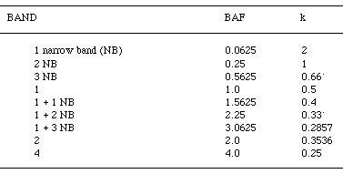
- When checking borderline trees by Relaskop (which self-corrects for slope), measure the slope angle (Ø) from the observer's eye to the centre of the tree at breast height, the breast high diameter d (cm) and the slope distance D (m). Then apply Formula 22 to determine the limiting distance (LD - m):

Values of k for the various bands and band combinations of a Relaskop are listed in Table 3.2.
Table 3.2 K values for Determining Limiting Distances when Angle Count Sampling Using a Standard Metric Spiegel Relaskop with the Brake Freed
Generally speaking, it is unnecessary to calibrate or check the calibration of either manufactured wedge prisms, which today are made from lenses of 'eyeglass' quality, or of the bands and band combinations of a Relaskop. However, if the prisms are cut locally, e.g. in a scientific workshop on a university campus, the user will need to calibrate each instrument. Calibration is best done in the laboratory . Recommended procedure is:
- Preferably sight to a flat target stood vertically (e.g. two clear, parallel lines a known distance apart drawn on a flat board) or, less preferably, to a target of circular cross section (e.g. drum or section of pipe of known diameter stood on end, etc.), and move backwards or forwards until the target is perfectly covered by the gauge (Relaskop, thumb, stick) or the image is perfectly displaced (wedge prism).
- Measure the width of the target (d) and the slope distance (D) from the eye to the target (for Relaskop with brake button depressed, thumb, or stick) or from the instrument to the target (for wedge prism).
- With the Relaskop, als0 measure the slope angle from the instrument to the target and correct the measured slope distance to its horizontal equivalent.
- Apply the appropriate calibration formula, namely:
