Forest Measurement and Modelling.
|
|
Stand table and frequency diagrams Forest Measurement and Modelling. |
     |
|
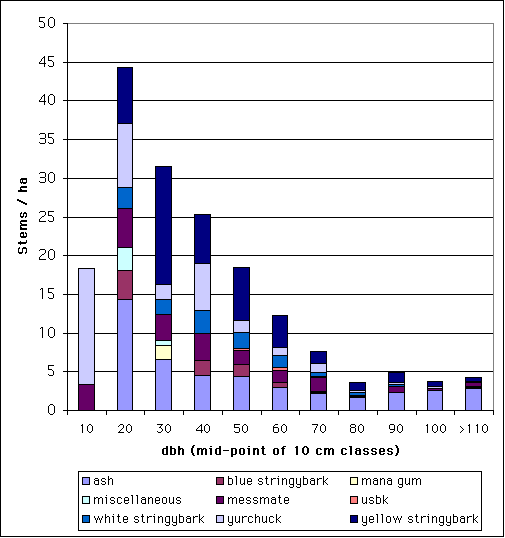
A stand table is a summary of the frequency of occurrence of trees by some classification system. A common system is a two-way classification by species and diameter class. The stand table can summarise information from hundreds of individual tree measurements into a simple table that a reader can quickly comprehend. To ensure maximum comprehension and to minimise the chance of misinterpretation, the classification system should follow some simple rules:
| |
| Frequency diagrams |
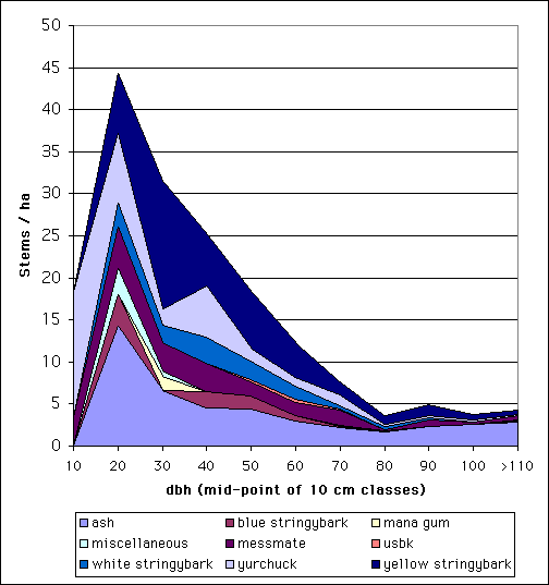
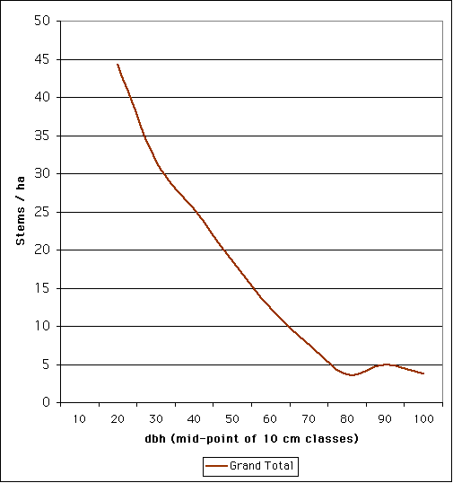
This information can also be presented in graphical form as a frequency diagram. Frequency diagrams take a variety of forms:
|
| Modelling the frequency curve |
The curve is often estimated by frequency distribution functions. In well-maintained plantations, for example, the frequency curve may approximate a normal distribution. In a normal distribution, the mean, mode and median sizes are all equal, and the distribution follows a bell shaped curve. Often however the frequency is not normally distributed. Where the distribution is skewed from normal (i.e. mean is not equal to median or mode) then a Beta function may be more appropriate for estimation. The a and b constants fix the minimum and maximum sizes respectively while m and n determine the shape of the distribution. The k constant is a scalar value to correct the overall frequency value. 
Many natural and uneven-aged forests do not approximate the normal distribution. Instead, these forests appear to follow a reverse-J distribution with many small trees and only a few large trees. In 1898, De Liocourt observed that the ratio between the number of trees in successive diameter classes was roughly constant for a particular forest. This observation lead to the development of a simple geometric series that estimated the number of trees in successive diameter classes. This series is based on the number of trees in the largest size class of interest (a) and the ratio of the next largest class to the largest class (q). If the largest size class (i) is classified as 0, and the next class as 1, ..., with the smallest class of interest being denoted as class n, then the frequency (F) of any class can be calculated as:  This produces the geometric sequence:   Applying De Liocourt's approach to the example frequency data from Eden results in a reasonable agreement (except for the smallest class). In this case, a was the frequency in the 100 cm class (3.80) and q was estimated as 1.35. Applying De Liocourt's approach to the example frequency data from Eden results in a reasonable agreement (except for the smallest class). In this case, a was the frequency in the 100 cm class (3.80) and q was estimated as 1.35. The values for a and q vary between forests and sites. Values for native forests in northeastern NSW have varied between 1.47 and 2 (e.g. Curtin, 1962). 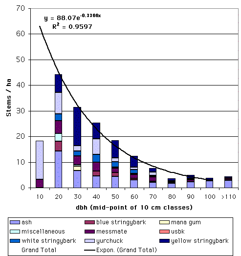 The advent of freely accessible computers for statistical analysis has allowed generalised and more powerful equations to be fitted to these frequency distributions. For example, a negative exponential curve fitted to the Eden data explained over 95% of the variation. The form of this equation is (where a0-a4 denote constants): The advent of freely accessible computers for statistical analysis has allowed generalised and more powerful equations to be fitted to these frequency distributions. For example, a negative exponential curve fitted to the Eden data explained over 95% of the variation. The form of this equation is (where a0-a4 denote constants):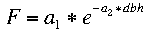 This can be transformed by taking the natural log to get a linear equation: 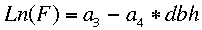 However, the most powerful equation form that is routinely fitted to this frequency distribution data is the Weibull model. This model can approximate normal and reverse-J distributions. The three-parameter form of the Weibull model includes three constants (a, b and c) which control the location, scale and shape (respectively) of the distribution: 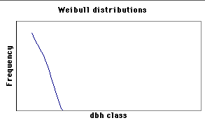 Where dbh > a and b, c > 0. |

|
[s_table.htm] Revision: 6/1999 |