 Histogram
 Polygon
 Curve
Curve
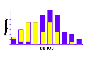
Species           10    20     30    40    50   60    70    80    90    100
                                    No. of trees

Euc. rossii    ``  2     1      1
Euc. maculosa      5     7     15     5     0    1     1
Euc. macrorhyncha                           1    5     7     2    0      1
A stand table summarises the information on a stand characteristic and facilitates manipulation of that information.
Stand tables are compiled following the enumeration or assessment of a stand. Compilation normally is on a unit area basis but it may be on a stand basis.
Class width, which should be specified, is usually held constant. Width depends on several factors including:
Measurement should always be consistent with the class limits. For example, if the limits are 10-12 cm (10.00-11.99), 12-14 cm, 14-16 cm, etc., enumeration should be to the nearest whole cm.
The trees may be measured and identified individually in the enumeration or they may be tallied by the gate or dot system or by some manually operated counter. A special coding system is necessary for mechanical data processing.
Once the stand table is compiled, the individual tree loses its identity and takes the central value of the class. This may give rise to anomalous results if class width is wide and frequency (number of trees per class) is low.
The size pattern of trees in a forest crop is usually described by three parameters - the mean, the variance and the type of distribution. These parameters are commonly established using a representative sample of trees drawn from the population.
Plotting the stand table data (frequency vs. class) on rectangular coordinate paper results in a FREQUENCY DIAGRAM which may take the form of a:
Histogram
Polygon
Curve
Knowledge of the distribution of tree diameters in forest crops is important to the forest manager because trees of different size may have different uses and monetary values. The distributions commonly used in forest management planning include the Normal, Beta and Weibull models.
The Normal distribution is characterised by a "bell shaped" curve with mean, mode and median all equal. It is described by the mean and the variance and may be predicted by reference to published tables of the normal deviate (Areas of a Standard Normal Distribution):
z = ( x-m ) /s.
The Beta function is:
Yx = k (x-a)m (b-x)nwhere Yx = frequency of trees / ha in diameter class x
k = scaling factor
a = smallest diameter in the stand
b = largest diameter in the stand
m and n = constants determining the shape of the distribution.
The constants are calculated using data collected from representative stands and applying techniques described in standard texts (e.g. Loetsch, Z^hrer and Haller, 1973).
The Weibull model is very flexible and has been used extensively in forestry for modelling diameter distributions. The complete model is:
Yx = cb^-1 [(x-a)/b] ^c-1 . Exp [-((x-a )/b)^c]and a, b and c are constants controlling the location, scale and shape respectively of the distribution.where x a, b, c > o, Yx and x are as defined above,
Forests around the globe differ in structure, i.e. the various species, sizes of tree and ages are grouped in different ways.
The structure of a stand is a result of both the growth habits of the species represented and the ecological conditions and management practices under which the stand originated and developed.
The two typical stand structures are even-aged and uneven-aged although under natural forest conditions all gradations between the two occur.
Even-aged forest, as used here, implies identical age of the component trees or such a small difference in age that, for practical purposes, it is unimportant, i.e. the difference in age between the trees does not affect the application of routine cultural treatments.
Uneven-aged forest may vary from a complete intermixture of species and age classes with no obvious boundaries between them, to forest with many age classes resulting from regeneration occurring in scattered patches over many years, to two-tiered/storeyed high forest where the age classes are more or less distinct.
Even-aged forest crops are much easier to describe than uneven-aged crops because the frequency distributions tend to be normal and the variances are small. Thus, a measure of average tree size (diameter, height, volume, etc.) is meaningful. This is not the case with uneven-aged forests for which frequency distributions are much less easily predicted and average tree size has little meaning.
In an unthinned even-aged stand, the frequency curve of dbhob approximates a statistically normal curve. The distribution is usually skewed normal. 
The distribution of tree heights in plantations is normal or slightly skewed normal. Crops on fertile sites, unthinned crops and shade tolerant species exhibit height distributions showing greater variation than is found in crops on poorer sites, purposively thinned stands and stands of light demanding species.
Normality can be demonstrated mathematically or by plotting cumulative frequency percent against size (dbhob) on arithmetic probability paper. A normal distribution plots as a straight line.
Several factors such as the species and its growth habits, age, site factors and action by man (e.g. thinning) determine how closely a stand approaches normality. A bi-modal distribution may even be found in a managed forest if thinning has selectively removed trees in some size classes.
As stated, the general pattern of distribution of trees by size class in an even-aged stand is skewed normal. If the sorting is slow, the frequency curve in the early stages of stand development may be reverse J-shaped, i.e. positively skewed with the greatest number of trees occurring in the smaller classes. 
As the stand ages, the curve may shift to the right until eventually, in an over-mature stand, a negatively skewed distribution may be found. 
Thus, the frequency distribution of trees varies both between stands and within a stand over time.
Work by Gates, McMurtrie and Borough (Aust. For. Res., 1983, 13: 267-70) based on spacing trials of Pinus radiata at Mt. Burr indicate distributions whose skewness initially becomes more negative with time but subsequently reverses direction, becomes positive, and then continues to become more positive with time. They suggest competition between neighbouring trees as a possible explanation for these trends.
If the distribution is normal, or likely to be so, forecasts of the diameter distribution at a future date (needed for management planning) will not be difficult provided the number of trees is known and the mean and standard deviation of the distribution can be forecast (straightforward if the stand has been measured periodically in the past). Unfortunately, silvicultural treatment often alters the distribution and complicates forecasting, the extent depending on the kind, severity and frequency of treatment. For example, periodic thinning either from above or below will continually upset normality and make forecasting difficult. Free thinning on the other hand may have little effect.
Stand tables for uneven-aged stands cover a considerable range of both age and size. The frequency distribution for diameter (dbhob) in such stands is typically reverse J-shaped, the frequency decreasing with increase in diameter. 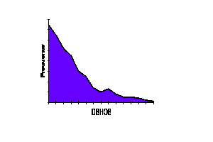
Evidence (Assmann, 1970: "The Principles of Forest Yield Study", p. 447+; Carron, unpubl. data) suggests that the J-shaped curve is an oversimplification and that, in fact, it is made up of a number of even-aged unimodal distributions. 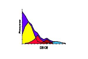
In 1898, De Liocourt observed in selection forests in France that the ratio between the number of trees in successive diameter classes was roughly constant for a particular forest, but varied from one forest to another. His observations were subsequently confirmed in many kinds of uneven-aged forests throughout the world. De Liocourt's model, a negative exponential model, applies particularly in mixed forests where the age classes and recruitment by natural regeneration are continuous.
Supposing we represent the ratio by 'q', then the number of trees in successive diameter classes is represented by a descending geometric series of the form:
aq^n-1, aq ^n-2, .................aq^3, aq^2, aq, a
where 'a' is the number of trees in the largest size class of interest
and 'n' is the number of classes.
Enumeration of a stand of mixed eucalypts at Pine Creek State Forest in northern NSW , 20 km south of Coffs Harbour, yielded the following data:-
Dbhob Class (cm)  10-20  20-30  30-40  40-50  50-60  60-70  70-80
Freq. / ha        119.4   55.4   35.1   22.5   10.9    5.9    4.4
Freq. / ha 119.4 68.9 39.7 22.9 13.2 7.6 4.4
For such a geometric series, if the logarithm of the frequency in successive classes is plotted against size of class on rectangular coordinate paper, or if frequency is plotted against size of class on semi-log paper, the distribution can be represented as an exponential curve of the form:
y = ke^-ax
where y = number of trees in diameter class x
e = base of natural logs (2.718)
and k and a are constants for a given diameter distribution.
The constants k and a in the equation above vary between forests and with site. 'k' reflects the occurrence of seedling regeneration and tends to be large in forests containing prolific seed-bearing tree species while 'a' determines the relative frequencies of successive diameter classes. A high 'a' is associated with high mortality between classes and is likely to occur in stands comprising light demanding (shade intolerant) tree species.
Thus, log y = log k - ax log ei.e. log y = k1 + k2 x
where k2 = - a log e.
The regression equation satisfying the Pine Creek data presented earlier is:
Log y = 2.3954 - 0.024 121x.
Predicting from this equation gives the following distribution:
Dbhob Class (cm)  10-20  20-30  30-40  40-50  50-60  60-70  70-80

Freq. / ha        108.0   62.0   35.6   20.4   11.7    6.7    3.9
Again, agreement with the actual distribution is good!
The Pine Creek data suggest a 'q' value of 1.73. Jacobs (1955 used a 'q' value of 2 for deriving simple stocking guides in uneven-aged eucalypt forest of the type found at Pine Creek. However, Curtin (1962) has proposed a value of 1.47 for maximum production in uneven-aged blackbutt stands in New South Wales.
Work by Carron (unpublished) suggests that seeking a constant 'q' in management may be unrealistic and misleading. Carron found that 'q' values in a well managed forest need not be constant over all diameter classes, and reports from other countries indicate that many truly all-aged stands do not in any way even approximate this type of distribution.
IndexHelp
Authors
| Document URL | http://online.anu.edu.au/Forestry/mensuration/STANDTAB.HTM |
| Editor | Cris Brack © |
| Last Modified Date | Fri, 9 Feb 1996 |
